Random Graph Generator

People have been talking about big data nowadays, and most of the big data problem I have encountered in real-world situations involve graphs.

Social network?

Biological network?

Financial network?

Graph is defined, in simple terms, as a set of nodes and a set of edges connecting these nodes. We can see that the situations above can be easily represented by graphs.

One problem researchers are concerned with is how to generate a graph so that they can test if their wonderful algorithms work on graphs. However, the algorithm to generate a random graph is a wonderful algorithm itself.

But what is the graph like?

Take Linkedin for example. If you are a recruiter or a sales person, you might have thousands of connections since that is simply your job to be social. But if you are a geek or a new graduate, you probably do not know many people out there and have only a few connections that are either your classmates or advisors. The graph is very unbalanced, where some people have many connections while some others have few. Theoretically, the distribution is called Power law.

How can we generate such a graph?

Barabási–Albert model is probably one of the most popular models to generate a graph with power law distribution. It employs preferential attachment mechanism to add new nodes. Preferential attachment means that the more connected a node is, the more likely it is to receive new links. When a new node comes into the graph, the probability of it attaching to an existing node is proportional to the degree of that existing node.

The process sounds very intuitive, since all we have to do is a for loop where it adds a new node to the graph and corresponding edges based on preferential attachment mechanism.

1 - Initialization

def generate_graph(node_size, avg_degree=None):
    # initialize an empty graph
    # each index represents a node and its neighbors
    graph = [[] for _ in range(node_size+1)]
    # endpoints, used for preferential attachment
    endpoints = []
    # avg_degree is the number of edges of newcomer that will be added to graph
    if avg_degree is None:
        avg_degree = 2

node_size is the size of the graph, that is, the total number of nodes. graph is a 2-d list that stores the nodes and all their neighbors. endpoints is used to replicate a node as many times as its degree. avg_degree is the default degree of a new node. With this we can make sure no one is alone and they have at least two friends.

2 - Seed graph

    # generate a complete graph as the seed graph, choose the seed_size so that each node has avg_degree neighbors in the seed graph
    seed_size = 2 * avg_degree + 1
    for i in range(1, seed_size):
        for j in range(i+1, seed_size+1):
            if i != j:
                graph[i].append(j)
                graph[j].append(i)
                endpoints.append(i)
                endpoints.append(j)

To apply preferential attachment, we need a seed graph so that we have some old nodes to attach new nodes to. We set the seed graph as a complete graph, that is, every node is connected to every other node. To make sure the avg_degree is also the same in the seed graph, we need to choose the seed_size according to seed_size = 2 * avg_degree + 1.

3 - Add new nodes

	# generate the entire graph
    for new_comer in range(seed_size+1, node_size+1):
        old_friends = select_elements(endpoints, avg_degree)
        for old_friend in old_friends:
            graph[new_comer].append(old_friend)
            graph[old_friend].append(new_comer)
            endpoints.append(new_comer)
            endpoints.append(old_friend)

This is the juicy part of the whole algorithm. Let’s follow the procedure step by step. For a newcomer, we select avg_degree old friends for it, and we update the graph. Besides, we add them to endpoints for each pair of new_comer and old_friend. What is the use of endpoints? Let’s see how it is used in the function select_elements.

In select_elements, we want to choose avg_degree elements with probability proportional to their degrees. By replicating a node as many times as its degree in endpoints, and choosing randomly from endpoints, we guarantee the property of preferential attachment. For example, for a complete graph (1, 2, 3), its endpoints should be like [1,1,2,2,3,3], because each node has degree 2. Another problem in select_elements is since there are duplicates in endpoints, and you have to repeat until you have chosen enough DIFFERENT nodes from endpoints.

def select_elements(endpoints, avg_degree):
    """
    select avg_degree elements from endpoint, without duplicate values
    """
    result = set()
    while len(result) < avg_degree:
        result.add(random.choice(endpoints))
    return result

4 - Plot degree distribution

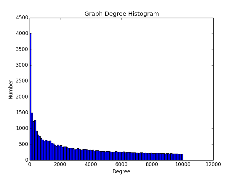
    pyplot.hist(endpoints, bins=100)
    pyplot.title("Graph Degree Histogram")
    pyplot.xlabel("Degree")
    pyplot.ylabel("Number")
    pyplot.show()

This part of code simply plots out the degree distribution of the graph using endpoints, as seen below.

This is an explanation of how to generate a power law graph using BA model. You are welcome to check out the code here. The final version might be a little different since I keep refininig it.

Thank you for reading :)